
Ask a shop when a new order can ship and the honest answer is often a shrug and a guess. The machines look busy, the planner has a feel for it, and the date that comes out is a hopeful round number. Two weeks later the order is late — not because anyone worked slowly, but because the machine it needed was quietly committed to three other jobs the whole time. Machine capacity planning replaces that shrug with two numbers per machine, and a percentage that makes the answer obvious.
This guide is for planners and production managers who schedule work across shared machines and want to promise dates they can keep. It covers what capacity planning is, how load and capacity are calculated, how to read loading percentage, and how Fast Planning Software shows it. Every number below is illustrative — used to make the arithmetic clear, not drawn from any specific plant. For the wider picture, start with the pillar guide, what is production planning software?
Scheduling decides the sequence; capacity planning tells you whether that sequence fits. If you want the scheduling half — priority, Gantt boards, sequencing rules — read the production scheduling guide. This article focuses on the load-versus-capacity arithmetic underneath it.
1. What machine capacity planning actually is
Machine capacity planning is the practice of comparing, for each machine or work centre, the work assigned to it against the work it can do in a period — so a plant knows whether its plan actually fits the machines it has, before it commits to dates. It answers the question every scheduler eventually hits: we have the orders and the material, but can the machines physically do this in the time we have?
It rests on two numbers, and everything else is derived from them:
- Load — the total hours of work assigned to a machine for the period. It comes from the operations routed to it: each operation's standard cycle time multiplied by the quantity, plus its setting (changeover) time.
- Capacity — the hours the machine actually has for the period. It comes from the shifts it runs, less planned downtime such as maintenance.
Compare the two — usually as a loading percentage — and the plant can see which machines are the constraint and which have room, while there is still time to do something about it. Skip it, and overloads only reveal themselves as missed dates. See Machine Loading & Capacity.
2. Load vs capacity — the two numbers
Getting these two right is the whole game, and each hides a common mistake.
| Aspect | Load (work assigned) | Capacity (work available) |
|---|---|---|
| Built from | Operations routed to the machine | Shifts the machine runs |
| Formula | (cycle time × qty) + setting time, summed | Shift hours × days, less planned downtime |
| Common mistake | Forgetting setting/changeover time | Assuming 100% of clock time is available |
| Grows when | More orders, bigger batches, more setups | You add a shift or a machine |
| Units | Hours (for the period) | Hours (for the same period) |
Two subtleties matter. First, setting time is part of load: a machine that changes over ten times a day can lose hours to setup that never appear if you count only cycle time — which is why grouping similar jobs to share a setup frees real capacity. Second, capacity is not the clock: a single 8-hour shift is not 8 hours of available machining once you subtract planned maintenance, tool changes and breaks. Capacity planning is only as honest as these two inputs; the standard cycle and setting times captured on each process sheet are what make the load figure trustworthy.
3. Calculating machine loading percentage (worked example)
Loading percentage is simply load ÷ capacity × 100. The value is in doing it per machine, so the comparison is like-for-like. Here is a worked example across four machines for one week — all figures illustrative:
| Machine (illustrative) | Load (hrs) | Capacity (hrs) | % loading | Reading |
|---|---|---|---|---|
| Turning centre A | 46 | 40 | 115% | Overloaded — the bottleneck |
| Milling B | 38 | 40 | 95% | Fully committed, little slack |
| Grinding C | 28 | 40 | 70% | Room to absorb more work |
| Turning centre D | 24 | 40 | 60% | Under-used — a levelling target |
The percentage does the work a raw hours figure cannot. Turning centre A at 115% is trying to do 46 hours of work in a 40-hour week — it is 6 hours short and will make something late unless the plan changes. Turning centre D at 60% has 16 spare hours. If A and D can run the same operations, moving roughly 6 hours of work from A to D brings A down to about 100% and lifts D to about 75% — the plant's total output is unchanged, but now every machine can keep the plan. That single move is the essence of capacity planning, and we will return to it under load levelling.
4. Finding the bottleneck
A bottleneck is the machine whose capacity constrains the whole plant's output — the one loaded well over 100% while others have room. It matters out of all proportion to its size, for a simple reason: the plant can only ship as fast as its bottleneck runs. Everything about capacity planning eventually points at finding it early.
- The bottleneck sets the realistic date. If turning centre A is the constraint, no promised date is credible unless A has the hours — the other machines waiting on A are not the limit.
- Time lost on the bottleneck is lost for the plant. An hour of breakdown or a slow setup on A is an hour of finished output the whole line never gets back; the same hour lost on an under-loaded machine costs nothing.
- The bottleneck can move. Relieve A and the constraint may shift to milling B at 95%. Capacity planning is continuous because the bottleneck is not fixed.
A machine loading report that ranks machines by loading percentage makes the bottleneck the top row — visible before the schedule is committed, not discovered when the order is already late.
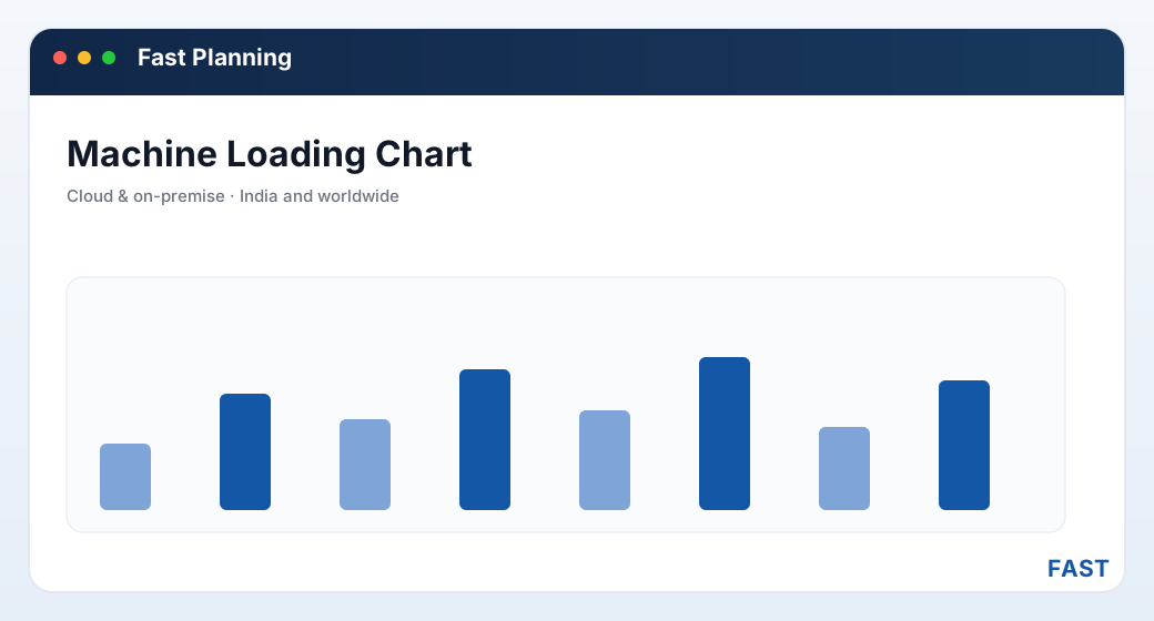
Ranked by loading percentage, the bottleneck is the top bar crossing the 100% line — visible before the week starts. Figures shown are illustrative.
5. Projected availability and pending work
Loading percentage tells you a machine is full; projected availability tells you when it will next be free. It is the forecast built from the pending work already loaded onto a machine — read against a loading report, it is what turns a promised date from a guess into a defensible commitment.
The logic is straightforward. If turning centre A is loaded solid for the next six working days, an operation that needs A cannot start until day seven, however urgent it is — unless something already on A is pushed aside. So when a customer asks for a date, the honest answer is not "the machine is free now" but "the machine has this much pending work, so the earliest this operation can start is here." Reading load against pending work lets a planner:
- Promise a real date — based on when the needed machine actually clears, not on optimism.
- Decide whether to expedite — see exactly what would have to move to pull an urgent order forward, and at what cost to other jobs.
- Spot forward overloads — a machine that is fine this week but solidly booked three weeks out, while there is still time to add capacity.
This is why a machine loading report is read two ways: current load for this week's bottleneck, and pending load for the promise you make on the next order.
6. Load levelling across machines and shifts
Finding an overload is only half the job; load levelling is fixing it — spreading work so no machine drowns while another idles. There are three levers, in rough order of preference:
- Shift operations to a capable, less-loaded machine
- Uses resource priority — preferred vs fallback
- No new cost; just better use of what you have
- Raises the capacity side of the ratio
- For a genuine, sustained overload
- Costs money — use when moving work is not enough
- Move non-urgent work to a lighter week
- Smooths a temporary spike
- Pairs with priority on the Gantt board
- Run similar jobs back to back
- Pay changeover once, not repeatedly
- Frees hidden capacity on the bottleneck
Take the earlier example: turning centre A at 115% (46h/40h) and turning centre D at 60% (24h/40h). The planner moves roughly 6 hours of A's operations to D using resource priority. A drops to about 100% (40h), D rises to about 75% (30h), and both are now inside capacity — the same total work, but a plan every machine can keep, with no overtime. Only if the whole cell were over 100% would adding a shift come into play. All figures illustrative.
7. Common traps that hide an overload
Capacity planning fails quietly, in predictable ways. Watch for these:
- A machine with frequent changeovers loses real hours to setup
- Load that ignores setting time understates the true load
- Capture setting time on the process sheet, not just cycle time
- A shift is not fully available once maintenance and breaks are out
- Overstated capacity hides an overload until it bites
- Subtract planned downtime to get honest available hours
- Total plant load can look fine while one machine drowns
- An average hides the bottleneck completely
- Always read loading per machine and per work centre
- A machine free today may be booked solid next week
- Promising against current, not projected, availability slips dates
- Read pending work before you commit a date
8. How Fast Planning Software implements capacity planning
Fast Planning Software is the MRP and production-planning product of the Fast Suite, built in Pune by Improsys under the Fast Technology brand, deployable cloud or on-premise for manufacturers across India and worldwide. It turns the arithmetic above into live screens:
| Capability | How Fast Planning Software does it |
|---|---|
| Load from operations | Each work order's operations carry standard cycle and setting times from the process sheet, so load is built from real durations — cycle time times quantity plus setting — not estimates. See process sheets & routing. |
| Daily machine loading | A machine loading report shows the daily load on each machine or work centre, and its loading as a percentage, so the bottleneck is the top of the list. See machine loading & capacity. |
| Loading on pending work | The loading report reads against pending work to project when a busy machine will next be free — so a promise date is based on when the machine actually clears. |
| Projected availability | Pending load projects each machine's next free window, so a planner can promise a realistic date and see what would have to move to expedite. |
| Load levelling | Resource priority moves operations to a capable, less-loaded machine, and re-sequencing on the Gantt board smooths a temporary spike — so the load levels without overtime where possible. |
| Actuals close the loop | The floor books actual run and setting times by barcode, so next period's load figures use times the shop floor really hits — feeding plan vs actual and OEE. |
See the load on every machine before you promise a date.
Fast Planning builds load from the real cycle and setting times on your process sheets, shows daily load and % loading per machine, and projects availability from pending work. Because it shares one platform with the rest of the Fast Suite, the same work orders you load flow to Fast Production and feed plan-vs-actual and OEE — so tomorrow's capacity figures use the times your floor actually hits.
9. Frequently asked questions
See the load on your own machines
A 30-minute demo — your process times, your machines, daily load and % loading with projected availability. No generic slideshow.